Summarizing Data:
PRECISION
OF MEASUREMENT continued
 MEASURES
OF VALIDITY
MEASURES
OF VALIDITY
Update Oct 2011: view this slideshow on validity and reliability for an overview of the important principles.
If you haven't read the general
introduction to precision of
measurement, do so now. A variable or measure is valid if its
values are close to the true values of the thing that the variable or
measure represents. In plain language, it's valid if it measures what
it's supposed to. This concept of validity is known as concurrent
validity, and it's the only one I will deal with here.
Measures of validity are similar to measures
of reliability. With reliability, you compare one measurement of
a variable on a group of subjects with another measurement of the
same variable on the same subjects. With validity, you also compare
two measurements on the same subjects. The first measurement is for
the variable you are interested in, which is usually some
practical variable or measure. The second measurement is for a
variable that gives values as close as you can get to the true values
of whatever you are trying to measure. We call this variable the
criterion variable or measure. The three main measures of
reliability--change in the mean, within-subject variation, and retest
correlation--are adapted to represent validity. I call them the
estimation equation, typical
error of the estimate, and validity
correlation. There is also a measure of limits of
agreement. I have a little to say on validity
of nominal variables (kappa coefficient, sensitivity, and
specificity), and I finish this page with a spreadsheet
for calculating validity.
You will find that correlation has a more prominent role in
validity than in reliability. Most applications of validity involve
differences between subjects, so the between-subject standard
deviation stays in the analysis and can be expressed as part of a
correlation. In contrast, most applications of reliability involve
changes within subjects; when you compute changes, the
between-subject variation disappears, and with it goes
correlation.
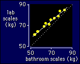 Let's
explore these concepts with an example similar to the one I used for
reliability. Imagine you are a roving applied sport scientist, and
you want to measure the weight of athletes quickly and easily with
portable bathroom scales. You check out the validity of the bathroom
scales by measuring a sample of athletes with the scales and with
certified laboratory scales, as shown in the figure. I've shown only
10 points, but in practice you'd use probably 20 or so, depending on
how good the scales were.
Let's
explore these concepts with an example similar to the one I used for
reliability. Imagine you are a roving applied sport scientist, and
you want to measure the weight of athletes quickly and easily with
portable bathroom scales. You check out the validity of the bathroom
scales by measuring a sample of athletes with the scales and with
certified laboratory scales, as shown in the figure. I've shown only
10 points, but in practice you'd use probably 20 or so, depending on
how good the scales were.
Note that I have assigned the observed value of the variable to
the X axis, and the true value to the Y axis. That's because you want
to use the observed value to predict the true value, so you must make
the observed value the independent variable and the true value the
dependent variable. It's wrong to put them the other way around, even
though you might think that the observed value is dependent on the
true value.
Estimation
Equation
The dotted line in the figure
represents perfect validity: identical weights on the bathroom and
lab scales. The solid line is the best straight line through the
observed weights. Notice how the lighter weights are further away
from the true value. That trend away from the true value is
represented by the estimation or calibration equation.
Any deviation away from the dotted line represents a
systematic offset.
Notice also that a straight line is a pretty good way to relate
the observed value to the true value. You'd be justified in fitting
a straight line to these data and using it to predict the true
weight (lab scales) from the observed weight (bathroom scales) for
any athletes on your travels.
By the way, you won't always get a straight line when you plot
true values against observed values. When you get a curve, fit a
curve! You can fit polynomials or more
general non-linear models. You know you
have the right curve when your points are scattered fairly evenly
around it. Use the equation of the curve to predict the true values
from the observed values.
You can also use a practical measure that looks nothing like the
criterion measure. For example, if you are interested in predicting
body fat from skinfold thickness, the practical measure would be
skinfold thickness (in mm) measured with calipers, and the criterion
measure could be body fat (as percent of body mass) measured with
dual-emission X-ray absorptiometry (DEXA). You then find the best
equation to link these two measures for your subjects.
There are sometimes substantial differences in the estimation equation for
different groups of subjects. For example, you'd probably find substantially
different equations linking skinfold thickness to body fat for subjects differing
in such characteristics as sex, age, race, and fitness. Sure, you can derive
separate equations for separate subgroups, but it's usually better to account
for the effect of subject characteristics by including them as independent variables
in the estimation equation. For that you need the technique of multiple
linear regression, or you could even go to exotic multiple non-linear models.
A stepwise or similar approach will allow
you to select only those characteristics that produce substantial improvements
in the estimation of the criterion.
Typical
Error of the Estimate
Notice how the points are scattered
about the line. This scatter means that any time you use the line to
estimate an athlete's true weight from the bathroom scales, there
will be an error. The magnitude of the error, expressed as a standard
deviation, is the typical error of the estimate: it's the
typical error in your estimate of an athlete's true weight. We've met
this term already as the standard error of the
estimate. I used to call it the standard deviation of the
estimate. Now I prefer typical error, because it is the
typical amount by which the estimate is wrong for any given subject.
In the above example, the typical error of the estimate is 0.5
kg.
The typical error of the estimate is usually in the output of
standard statistical analyses when you fit a straight line to data.
If you fit a curve, the output of your stats program might call it
the root mean-square error or the residual
variation. Some stats programs provide it in the squared form, in
which case you will have to take the square root. Your program almost
certainly won't give you confidence limits for the typical error, but
you should nevertheless calculate them and publish them. See the
spreadsheet for confidence
limits.
In the sections on reliability, I explained that the within-subject variation
can be calculated as a percent variation--the coefficient of variation--by analyzing
the log of the variable. The same applies here: take logs of your true and observed
values, fit a straight line or curve, then convert the typical error of the
estimate to a percent variation using the same formula as for reliability. See
reliability calculations for the formula. Analysis
of the logs is included in the validity spreadsheet. In
the above example the standard deviation is 0.7%. Expressing the standard deviation
as a percent is particularly appropriate when the scatter about the line or
curve gets bigger for bigger untransformed values of the estimate. Taking logs
usually makes the scatter uniform. See log transformation
for more.
New-Prediction Error
If a validity study has a small sample size
(<50 subjects), the typical error of the estimate is accurate only for the
subjects in the validity study. When you use the equation to predict
a new subject's criterion value, the error in the new estimate--let's
call it the new-prediction error--is larger than the original typical
error of the estimate. Why? Because the calibration equation (intercept and
slope) varies from sample to sample, and the variation is negligible only for
large samples. The variation in the calibration equation for small samples therefore
introduces some extra uncertainty into any prediction for a new subject, so
up goes the error. The uncertainty in the intercept contributes a constant additional
amount of error for any predicted value, but the error in the slope produces
a bigger error as you move away from the middle of the data. Your stats program
automatically includes these extra errors when you request confidence limits
for predicted values. You will find that the confidence limits get further away
from the line as you move out from the middle of the data. The effect is noticeable
only for small samples or only for predicted values that are far beyond the
data.
So, exactly how big is the error in a predicted value based on a validity or
calibration study with a small sample size? If you have enough information from
the study, you can work out the error accurately for any predicted value. Obviously
you need the slope, intercept, and the typical error of the estimate. You also
need the mean and standard deviation of the practical variable (the X values).
I've factored all these into the formulae for the upper and lower confidence
limits of a predicted value in the spreadsheet for analysis
of a validity study. I've also included them in the validity part of the
spreadsheet for assessing an individual. (In
that spreadsheet I've used the mean and standard deviation of the criterion
or Y variable, because it's convenient to do so, and the difference is negligible.)
When you don't have access to the means or standard deviations from the validity
study, you can work out an average value for the new-prediction error, on the
assumption that your new subject is drawn randomly from the same population
as the subjects in the validity study. One approach to calculating this error
is via the PRESS statistic. (PRESS = Predicted REsidual Sums of Squares.)
I won't explain the approach, partly because it's complicated, partly because
the PRESS-derived estimate is biased high, and partly because I have better
estimates. For one predictor variable, the exact formula for the new-prediction
error appears to be the typical error multiplied by root(1+1/n+1/(n-3)), where
n is the sample size in the validity study. I checked by simulation that this
formula works. I haven't yet worked out the exact formula for more than one
predictor variable, but my simulations show that the typical error multiplied
by root[(n-1)/(n-m-2)] is pretty good, where m is the number of predictor variables.
Researchers in the past got quite confused about the concept of error in the
prediction of new values. They used to split their validity sample into two
groups, derive the estimation equation for one group, then apply it to the second
group to check whether the error of the estimate was inflated substantially.
That approach missed the point somehow, because the error was bound to be inflated,
although they apparently didn't realize that the inflation was usually negligible.
And whether or not they found substantial inflation, they should still have
analyzed all the data to get the most precise estimates of validity and the
calibration equation. The PRESS approach has a vestige of that data-splitting
philosophy. Not that it all matters much, because most validity studies have
more than 50 subjects, so the new-prediction error from these studies is practically
identical to the typical error of the estimate.
A final point about the new-prediction error: don't use it to compare the validity
of one measure with that of another, even when the sample sizes are small and
different. Use the typical error, which is an unbiased and unbeatable measure
of validity, no matter what the sample size. (Actually, it's the square of the
typical error that is unbiased, but don't worry about that subtlety.)
Non-Uniform Error of the Estimate
You will recall that calculations for reliability
are based on the assumption that every subject has the same typical error, and
we used the term heteroscedasticity to
describes any non-uniform typical error.
The same assumption and terminology underlies calculations for the validity,
and the approach to checking for and dealing with any non-uniformity is similar.
Start by looking at the scatter of points on the plot of the estimation equation.
If every subject has the same typical error of the estimate, the scatter of
points, measured in the vertical direction on the graph (parallel to the Y axis),
should be the same wherever you are on the line or curve. It's difficult to
tell when the points lie close to the line or curve, so you get a much better
idea by examining the difference between the observed and the predicted values
of the criterion for each subject. These differences are known as the residuals,
and it's usual to plot the residuals against predicteds values. I have provided
such a plot on the spreadsheet, or click
here to see a plot from a later section of this text. If subjects in one
part of the plot have a bigger scatter, they have a bigger typical error (because
the standard deviation of the residuals is the typical error). The calculated
typical error of the estimate then represents some kind of average variation
for all the subjects, but it will be too large for some subjects and too small
for others.
To get an estimate of the typical error that applies accurately to all subjects,
you have to find some way to transform the criterion and practical measures
to make the scatter of residuals for the transformed measures uniform. Once
again, logarithmic transformation often reduces non-uniformity of the scatter
in situations where there is clearly more variation about the line for larger
values of the criterion. A uniform scatter of the residuals after log transformation
implies that the typical error, when expressed as a percent of the criterion
value, is the same for all subjects; the typical error from analysis of the
log-transformed measures then gives the best estimate of its magnitude. I have
included an analysis of the log-transformed measures in the spreadsheet, although
for the data therein it is clear that the scatter of residuals is more uniform
for the raw measures than for the log-transformed measures.
If you fit a curve rather than a straight line to your data, the standard deviation
of the residuals (the root mean square error) still represents the typical error
in the estimate of the criterion value for a given practical value. To estimate
the typical error from the spreadsheet might be too difficult, though, because
you will have to modify the predicted values according to the type of curve
you used. It may be easier to use a stats program. The typical error in the
output from the stats program will be labeled either as the SEE, the root mean-square
error, or the residual error. Some stats programs provide the typical error
as a variance, in which case you will have to take the square root.
When you have subgroups of subjects with different characteristics (e.g., males
and females), don't forget to check whether the subgroups have similar typical
errors. To do so, you should label the points for each subgroup in the plot
of residuals vs predicteds, because what looks like a uniform scatter might
conceal a big difference between the subgroups. If there is a big difference,
you shouldn't use a composite estimation equation for the two groups; instead,
you should derive separate equations and separate typical errors for each subgroup.
Validity Limits of
Agreement
By analogy with reliability
limits of agreement, we can define validity limits of
agreement as the 95% likely range or reference range for the
difference between a subject's values for the criterion and practical
measures. Let's try to understand this concept using the data in the
validity spreadsheet.
The data are from a validity study in which the practical measure
was body fat estimated using a Bod Pod, and the criterion measure was
body fat measured with a DEXA scan. The units of body fat are percent
of body mass (%BM). The limits of agreement (not shown in the
spreadsheet) are -2.9 to 7.9 %BM, or 2.5 ± 5.4 %BM. You can
interpret these numbers in two ways: there's a 95% chance that a
subject's "true" (DEXA) body fat is within 2.5 ± 5.4 %BF of his
or her Bod Pod value; or, if you measured a large number of subjects
in the Bod Pod, 95% of them would have a DEXA body fat within 2.5
± 5.4 %BF of their Bod Pod values. The value 2.5 in this
example is the mean of the criterion-practical difference (or the
difference between the means of the criterion and practical
measures); it is sometimes known as the bias in the practical
measure, but don't confuse this concept with the small-sample bias
I described in connection with
measures of reliability. The value ±5.4 on its own is
usually referred to as the limits of agreement; it is ±2.0x the
standard deviation of the criterion-practical difference (= 2.7). The
standard deviation of the criterion-practical difference is itself
known as the pure error or total error.
Limits of agreement are related to the typical error of the
estimate. When the slope of the estimation equation is exactly 1, the
pure error is the same as the typical error, so in this special case
the limits of agreement are twice the typical error. If the slope
differs from 1, the limits of agreement are greater than twice the
typical error. If the calibration equation is a curve rather than a
straight line, the limits of agreement will also be greater than
twice the typical error.
Advocates of limits of agreement encourage authors to plot the
criterion-practical differences against the mean of these measures
(or against the criterion). The resulting plot is similar to a plot
of the residuals against the predicteds from the analysis of the
estimation equation: if the estimation equation is a straight line of
slope close to 1, the criterion-practical differences are the same as
the residuals, and the mean of the criterion and practical is near
enough to the predicted value. The plot will therefore allow you to
check for heteroscedasticity. If the calibration equation is a
straight line with slope different from 1, or if it is a curve, the
scatter of points in the plot of the criterion-practical differences
will show a trend towards a straight line or a curve, so it will be
harder to tell if heteroscedasticity is present.
Validity limits of agreement suffer from problems similar to those
of reliability limits of agreement: they are harder to understand
than the typical error, and they are too large as a reference range
for making a decision about a subject's true (criterion) measurement.
The fact that the nature of the estimation equation affects the
magnitude of the limits is also a serious problem. Unfortunately some
authors have published limits of agreement without an estimation
equation or the typical error, so readers cannot properly assess the
practical measure and the published data cannot be used to
recalibrate the practical measure.
Validity
Correlation
The properties of the validity
correlation are similar to those of the retest
correlation. In particular...
- The correlation is a measure that combines within- and
between-subject variation. Within here refers to the
typical error of the estimate.
- The correlation gives you a good idea of how well the observed
value of a variable (weight on bathroom scales in our example)
retains the true rank order of subjects. Correlations >0.90 are
needed to retain reasonable order in the ranking. Don't use those
bathroom scales to assign athletes to competitive classes based on
weight unless the validity correlation is well above 0.90!
- The correlation is unaffected by any systematic offset.
- The correlation is sensitive to the nature of the sample used
to estimate it. For example, if the sample is homogeneous, the
correlation will be low. So whenever you interpret a correlation,
remember to take the sample into consideration.
- In contrast, the typical error of the estimate can be
estimated from a sample of subjects that is not particularly
representative of the population you want to study. You can
usually assume the estimate applies to any subject in the
population.
When it comes to calculating the validity correlation, you don't
have much choice: if you fit a straight line to the data, the
correlation is a Pearson correlation coefficient--there is no
equivalent intraclass correlation coefficient. If you fit a curve,
the stats program should provide you with a goodness-of-fit
statistic called the variance explained or the R-squared. Just
take the square root of this statistic and you have the equivalent of
the Pearson correlation coefficient.
An estimate of validity correlation can also be
obtained by taking the square root of the concurrent reliability
correlation. By concurrent reliability I mean the
immediate retest reliability, rather than the retest reliability over
the time frame of any experiment you may be planning. This
relationship between validity and reliability comes about because
reliability is the correlation of something with itself (and there is
error in both measurements), whereas validity is something correlated
with the real thing (so there is error in only one measurement). The
relationship can be derived from the definition
of correlation (covariance divided by product of standard deviations)
applied to the validity and reliability correlations.
The square root of concurrent reliability represents the maximum
possible value for validity. The actual validity correlation could be
less, because a measure can have high reliability and low validity.
To put it another way, a measure can produce nonsense
consistently!
Validity can be difficult to measure,
because the true value of something can be difficult to assay.
Measures other than the true value are called surrogates.
These measures usually result in underestimates of validity when they
are correlated with observed values, for obvious (I hope) reasons.
Here's an example. Body density obtained by underwater weighing is
often referred to as the gold standard for estimating percent body
fat, but it is only a surrogate for true percent body fat. So if you
are validating a skinfold estimate of body fat against the value
obtained by underwater weighing, the validity correlation will be
lower than if you validated the skinfold estimate against a more
accurate method than underwater weighing, for example, a DEXA scan.
Similarly the typical error of the estimate will be smaller when you
validate skinfolds against DEXA rather than underwater weighing.
Validity
of Nominal Variables
Validity of nominal
variables can be expressed as a kappa coefficient, a
statistic analogous to the Pearson correlation coefficient. Validity
of nominal variables doesn't come up much in sport or exercise
science--there's usually no question that you've got someone's sex or
sport right--but it's a big issue in clinical medicine, where yes/no
decisions have to be made about the presence of a disease or about
whether to apply an expensive treatment. In cases where the variable
has only two levels, clinicians have come up with other measures of
validity that are easier to interpret than correlations. For example,
sensitivity is the proportion or percent of true cases (people
with a disease) correctly categorized as having the disease by the
instrument/test/variable, and specificity is the proportion of
true non-cases (healthy people) correctly categorized as being
healthy. I have been unable to find or devise a simple relationship
between the kappa coefficient and these two measures. One of these
days...
Spreadsheet
for Calculating Validity
This spreadsheet shows an example
of a simple linear relationship between a practical measure (body fat
derived from body density, estimated with the Bod Pod) and a
criterion measure (body fat derived from dual energy X-ray
absorptiometry, or DEXA). To use the spreadsheet, replace these data
with your own data.
The spreadsheet estimates the calibration equation and the following measures
of validity: typical error of the estimate, new-prediction error, correlation
coefficient, and limits of agreement (but don't use them!). Analysis of log-transformed
data is included for estimation of errors as percents of the mean.
Go to: Next
· Previous
· Contents ·
Search
· Home
webmaster=AT=sportsci.org
· Sportsci
Homepage
Last updated 20 Aug 01