Compatibility Intervals and Magnitude-Based Decisions for Standardized Differences and Changes in Means Will G Hopkins Sportscience 23, 1-4, 2019
(sportsci.org/2019/MBDstzd.htm)
|
|||||
|
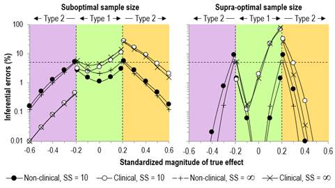
Update March 2023. In a recent article, Lin and Aloe (2021) referred to previous authors who devised approximations for the standard error of a standardized effect. It is evident that these can be derived by a first order approximation with calculus, as follows. The standardized mean effect SME = D/SD, where D is the difference or change in the means and SD is the standardizing standard deviation. Therefore, using first-order calculus, dSME = dD/SD – (D/SD2).dSD. If d represents the standard error, then the first term is the contribution to the standard error in the SMD arising from the standard error in the mean, and the second term is the contribution arising from the standard error in the standardizing standard deviation. The standard error of an SD is given by dSD = SD/Ö(2DF), where DF is the degrees of freedom of the standardizing SD (this Excel simulation checks this formula). Assuming these two terms are independent, the square of the standard error in the SME is given by (dD/SD)2 + [(D/SD2).SD/Ö(2DF)]2 = (dD/SD)2 + (D/SD)2/(2DF) = (dD/SD)2 + SME2/(2DF). This formula, and the formula for its degrees of freedom (given by the Satterthwaite approximation) are the same as those I arrived at with my simulations. However, my assertion that "such adjustment is unnecessary when the sample size of the standardizing SD is at least 30" is not correct; with a highly reliable dependent variable in a crossover or controlled trial, (dD/SD)2 could be comparable to or even smaller than SME2/(2DF), irrespective of sample size, if the SD is provided by the sample. Lin L, Aloe AM. (2021). Evaluation of various estimators for standardized mean difference in meta‐analysis. Statistics in Medicine 40, 403-426. A difference or change in a mean divided by an appropriate between-subject standard deviation (SD) is a dimensionless standardized statistic sometimes known as the effect size or Cohen's d. Standardization is a useful approach to assessing magnitude of an effect, when the dependent variable providing the difference or change in the mean is approximately normally distributed, and when there is no known relationship between the variable and health, wealth or performance that would allow assessment of meaningful effect magnitudes. For an example, consider a psychometric variable, agreeableness. Until researchers find a relationship of this variable with morbidity, mortality, success at work (e.g., chance of promotion) or at home (e.g., risk of divorce), standardization allows you to determine that an individual who is 2-4 SD below the mean has a very large level of disagreeableness and would need a treatment with a very large positive effect to bring him or her up to the mean value, according to the magnitude thresholds for standardized effects: <0.2, trivial; 0.2-0.6, small; 0.6-1.2, moderate; 1.2-2.0, large; 2.0-4.0, very large; >4.0, huge (Hopkins et al., 2009). The spreadsheets for analyzing differences and changes in means at this site have long suffered from failure to account for uncertainty in the standard deviation used to assess magnitude via standardization. I once thought the non-central t statistic was needed, but more recently I realized that the non-central t applies only to the special case of standardized effects where the standardizing SD can be expressed as a factor of the standard error of the difference or change in the mean. The non-central t would therefore not apply either to standardizing the difference in changes of the mean in controlled trials (where the pretest provides the standardizing SD) or to standardizing in any design with an SD from another sample. I also thought that dividing a mean by a standard deviation would produce a statistic with an unfathomable sampling distribution, such that compatibility (formerly confidence) limits and magnitude-based decisions (MBD; formerly magnitude-based inference) could be derived only by bootstrapping or full Bayesian analysis. Cumming and Finch (2001) had also reached some of these conclusions. Updating the Sportscience spreadsheets with bootstrapped compatibility limits and MBD was not a realistically implementable option. What to do? It occurred to me that the central limit theorem might be relied upon to give the usual t distribution for the standardized effect, perhaps even with sample sizes as low as 10, which is what sport scientists sometimes have to contend with. The breakthrough in deriving the t distribution was to realize that dividing by an SD is the same as multiplying by 1/SD. The standard error (SE) of the sampling distribution of the product could then be estimated from the SE of the mean and the SE of 1/SD, if an expression could be found for the latter. Simulation came to the rescue. In the accompanying first spreadsheet, I have used simulation to show that the fractional SE of 1/SD is given quite accurately by Ö(1/(2(DF-2)), where DF is the degrees of freedom of the SD. I arrived at this formula by starting with the fractional SD for the SD itself, which is given by Ö(1/(2(DF)). When I found that this formula underestimated the SE of 1/SD for small sample sizes, it was a simple matter to reduce the DF until the formula estimated the SE derived from simulated samples. I then had to derive a formula for combining the SE of the product of two independent statistics. This formula can be derived by statistical first principles, but I checked it with another spreadsheet. Next I used the resulting formula in a spreadsheet that simulates 10,000 studies of a standardized effect derived from a sample for the mean and another sample for the standardizing SD. In another spreadsheet I did the simulations using the population SD for the standardizing. Both spreadsheets are included in a single workbook (28 MB). I then varied values for the mean, the SD of the mean, the standardizing SD, and both sample sizes. I found that using the formula for the fractional SE of the SD rather than what I had derived for 1/SD gave 90% compatibility intervals with good coverage: the intervals included the true standardized effect at worst ~89% of the time (i.e., what I call the Type-0 error rate in the spreadsheet was at most ~11%). For the smallest sample sizes I investigated (10), the coverage was sometimes too conservative: an error rate down to ~6%. I therefore made the SE of the standardized effect slightly smaller by removing one of the terms in its formula, then included this simpler formula in the spreadsheet to check on the resulting error rates. The highest error rates of ~11% increased only slightly, while the lowest rates rose to ~8%. I considered this simpler formula to be a good compromise, and it made the job of updating all the relevant spreadsheets at Sportscience a little easier. Although the compatibility interval for the standardized effect has acceptable coverage of the true value for small sample sizes, the probabilities of the magnitude of the true value in MBD are based on the assumption of an underlying t distribution. The simulation spreadsheet allows investigation of this issue visually via a histogram of the sampling distribution of standardized effects and a Q-Q plot for normality. Non-normality is obvious in these figures when the sample size for the standardizing SD is 10 or even 20, especially when the mean standardized difference or change is substantial (greater than 0.20 or less than -0.20). Non-normality is also apparent in divergence of the 5th and 95th percentiles of the sampling distribution of the effect standardized with the sample SD from those standardized with the population SD. The assumption of normality is therefore visibly violated with small sample sizes for the standardizing SD. A reasonable approach to determining whether this non-normality renders the MBD probabilities untrustworthy is to determine the MBD error rates with the smallest sample sizes that sport scientists should ever use (10 for the mean and 10 for the standardizing SD), and compare the error rates with those in the second spreadsheet in the workbook, where the population SD is used to standardize and the sampling distribution is normal. By inserting appropriate values for the SD of the mean, I chose two scenarios: an effectively suboptimal sample size for the mean (one-fifth of the optimal, which would give 90% compatibility limits of ±0.48 rather than the optimal of ±0.20); and a supra-optimal sample size (approximately three times the optimal, which would give compatibility limits of ±0.12). These two scenarios correspond approximately to the sample sizes of 10+10 and 144+144 for the simulated controlled trials in the study of Hopkins and Batterham (2016), where the optimal sample size was 50+50. (I established the correspondence for a mean difference or change of zero.) Figure 1 shows the resulting MBD error rates.
The error rates for the standardizing sample size of 10 are remarkably similar to those for the population SD when the sample size for the mean is suboptimal. It is only with the supra-optimal sample size that the non-clinical Type-2 rate increases substantially and could be of concern for marginally substantial effects (10% rather than 5%). Given the narrow compatibility intervals with supra-optimal sample sizes, the Type-2 errors would not be associated with misapprehension about the true magnitude. The simulation spreadsheet can also be used to make adjustments to compatibility limits for a standardized effect that was derived previously with a small sample size for the standardizing SD. Make the sample size for the standardizing standard deviation in the spreadsheet the same as that in the previous study. Make the sample size for the mean difference or change in the spreadsheet approximately the same as that in the previous study. (If the previous study was a controlled trial, the sample size is near enough to the sum of the sample sizes in the two groups that provided the difference in the change in the means.) Next, make the mean difference or change in the spreadsheet a value that gives the mean standardized effect in the previous study. Now try different values of the standard deviation of the mean in the spreadsheet until you get the same mean compatibility limits derived with the population SD as those in the previous study. The mean compatibility limits that you now see in the spreadsheet coming from the sample standardizing standard deviation are a reasonable estimate of what the compatibility limits should have been, if the previous study had been analyzed appropriately. Use the upper and lower confidence limits to make a non-clinical or clinical magnitude-based decision. Finally, I have compared the compatibility limits derived from the sampling distributions of the mean effect standardized with the sample SD and with the population SD to address the question of the minimum sample size for the standardizing SD that allows the uncertainty in the SD to be ignored. The first surprising finding is that for a population mean of zero, the compatibility limits are negligibly wider (<5%) with a standardizing sample size of 10 than those with the population SD, regardless of the precision of the mean (varied by inserting different values of the population SD of the mean). The compatibility limits start to diverge when the population mean becomes small-moderate. Understandably, the divergence is less marked for greater uncertainty in the mean, because the standardizing SD contributes relatively less uncertainty to the standardized effect. With a sample size of 30 for the standardizing SD and with overall uncertainty in the standardized effect approximately equal to the mean (giving effects that are clear but approaching unclear), there is negligible difference between the compatibility limits using the sample vs population SD to standardize. The limits start to diverge when the overall uncertainty in the standardized mean is somewhat less than the standardized mean itself (e.g., mean standardized effect 1.00; 90%CL 0.69 to 1.37 using the sample SD; 0.74 to 1.26 using the population SD), but these effects would all be very clear, so there would be little concern about ignoring the uncertainty in the SD based on a sample of 30 or more. Several statistics other than differences and changes in means can be standardized: individual differences from the mean (e.g., the value of disagreeableness in the opening paragraph), individual changes (e.g., of an athlete's test score), and the standard deviation summarizing additional individual differences or changes in one group compared with a reference or control group (e.g., individual responses to a treatment). Compatibility limits of a standardized individual difference or change will depend on the error of measurement of the variable and could be derived by using the simulation spreadsheet to perform parametric bootstrapping. The uncertainty in the SD summarizing individual differences or changes is much greater than that of the mean difference or change (Hopkins, 2018), so it seems reasonable to neglect the contribution of uncertainty in the standardizing SD for this statistic, especially given that the overall sample size in a controlled trial needs to be at least 40 for reasonable accuracy of the compatibility limits of the SD representing individual responses. In conclusion, researchers can use an approximate t distribution to provide trustworthy compatibility intervals and decisions about the magnitudes of standardized differences and changes in means, even when the sample size for the standardizing SD is unavoidably as low as 10. The appendix provides formulae for the parameters of the t distribution, and the spreadsheets for analyzing differences and changes in means at the Sportscience site have now been updated with these formulae. When the sample size of the standardizing SD is at least 30, ignoring the uncertainty in the SD will not adversely affect decisions about magnitudes of standardized effects. References
Hopkins WG (2018). Design and analysis for studies of
individual responses. Sportscience 22, 39-51 Appendix
Here are the parameters of the approximate t distribution for a standardized effect. The mean, with the Becker (1988) adjustment to remove small-sample bias: (D/SD)(1-3/(4DFSD-1)), where D is the mean difference or change, SD is the standardizing standard deviation, and DFSD is the degrees of freedom of the SD. The standard error, Becker-adjusted: Ö[SE2+D2/DFSD/2](1-3/(4DFSD-1))/SD, where SE is the standard error of the mean effect. To give overall better coverage of the compatibility interval, the term omitted from the sum of the variances was +SE2/DFSD/2. The degrees of freedom, using the Satterthwaite (1946) formula: (SE2+D2/DFSD/2)2/(SE4/DFD+(D2/DFSD/2)2/DFSD), where DFD is the degrees of freedom of the SE. Published May 2019 |